31. Convolutional Network in TensorFlow
Convolutional Network in TensorFlow
It's time to walk through an example Convolutional Neural Network (CNN) in TensorFlow.
The structure of this network follows the classic structure of CNNs, which is a mix of convolutional layers and max pooling, followed by fully-connected layers.
The code you'll be looking at is similar to what you saw in the segment on Deep Neural Network in TensorFlow in the previous lesson, except we restructured the architecture of this network as a CNN.
Just like in that segment, here you'll study the line-by-line breakdown of the code. If you want, you can even download the code and run it yourself.
Thanks to Aymeric Damien for providing the original TensorFlow model on which this segment is based.
Time to dive in!
Dataset
You've seen this section of code from previous lessons. Here we're importing the MNIST dataset and using a convenient TensorFlow function to batch, scale, and One-Hot encode the data.
from tensorflow.examples.tutorials.mnist import input_data
mnist = input_data.read_data_sets(".", one_hot=True, reshape=False)

import tensorflow as tf

# Parameters
learning_rate = 0.00001
epochs = 10
batch_size = 128

# Number of samples to calculate validation and accuracy
# Decrease this if you're running out of memory to calculate accuracy
test_valid_size = 256

# Network Parameters
n_classes = 10  # MNIST total classes (0-9 digits)
dropout = 0.75  # Dropout, probability to keep units
Weights and Biases
# Store layers weight & bias
weights = {
    'wc1': tf.Variable(tf.random_normal([5, 5, 1, 32])),
    'wc2': tf.Variable(tf.random_normal([5, 5, 32, 64])),
    'wd1': tf.Variable(tf.random_normal([7*7*64, 1024])),
    'out': tf.Variable(tf.random_normal([1024, n_classes]))}

biases = {
    'bc1': tf.Variable(tf.random_normal([32])),
    'bc2': tf.Variable(tf.random_normal([64])),
    'bd1': tf.Variable(tf.random_normal([1024])),
    'out': tf.Variable(tf.random_normal([n_classes]))}
Convolutions

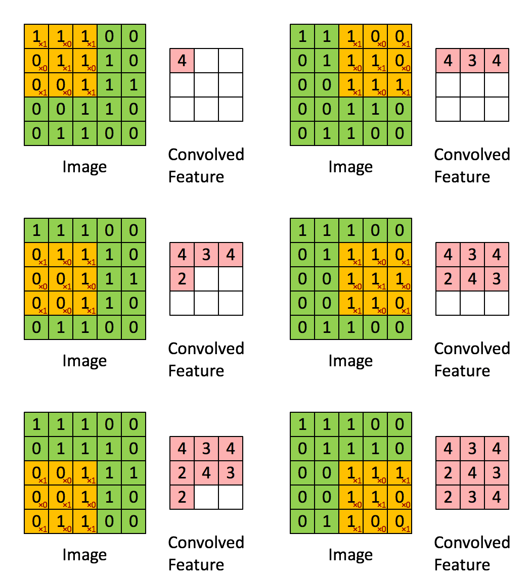
Convolution with 3×3 Filter. Source: http://deeplearning.stanford.edu/wiki/index.php/Feature_extraction_using_convolution
The above is an example of a
convolution
with a 3x3 filter and a stride of 1 being applied to data with a range of 0 to 1. The convolution for each 3x3 section is calculated against the weight,
[[1, 0, 1], [0, 1, 0], [1, 0, 1]]
, then a bias is added to create the convolved feature on the right. In this case, the bias is zero. In TensorFlow, this is all done using
tf.nn.conv2d()
and
tf.nn.bias_add()
.
def conv2d(x, W, b, strides=1):
    x = tf.nn.conv2d(x, W, strides=[1, strides, strides, 1], padding='SAME')
    x = tf.nn.bias_add(x, b)
    return tf.nn.relu(x)
The
tf.nn.conv2d()
function computes the convolution against weight
W
as shown above.
In TensorFlow,
strides
is an array of 4 elements; the first element in this array indicates the stride for batch and last element indicates stride for features. It's good practice to remove the batches or features you want to skip from the data set rather than use a stride to skip them. You can always set the first and last element to 1 in
strides
in order to use all batches and features.
The middle two elements are the strides for height and width respectively. I've mentioned stride as one number because you usually have a square stride where
height = width
. When someone says they are using a stride of 3, they usually mean
tf.nn.conv2d(x, W, strides=[1, 3, 3, 1])
.
To make life easier, the code is using
tf.nn.bias_add()
to add the bias. Using
tf.add()
doesn't work when the tensors aren't the same shape.
Max Pooling

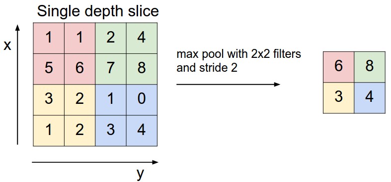
Max Pooling with 2x2 filter and stride of 2. Source: http://cs231n.github.io/convolutional-networks/
The above is an example of
max pooling
with a 2x2 filter and stride of 2. The left square is the input and the right square is the output. The four 2x2 colors in input represents each time the filter was applied to create the max on the right side. For example,
[[1, 1], [5, 6]]
becomes 6 and
[[3, 2], [1, 2]]
becomes 3.
def maxpool2d(x, k=2):
    return tf.nn.max_pool(
        x,
        ksize=[1, k, k, 1],
        strides=[1, k, k, 1],
        padding='SAME')
The
tf.nn.max_pool()
function does exactly what you would expect, it performs max pooling with the
ksize
parameter as the size of the filter.
Model

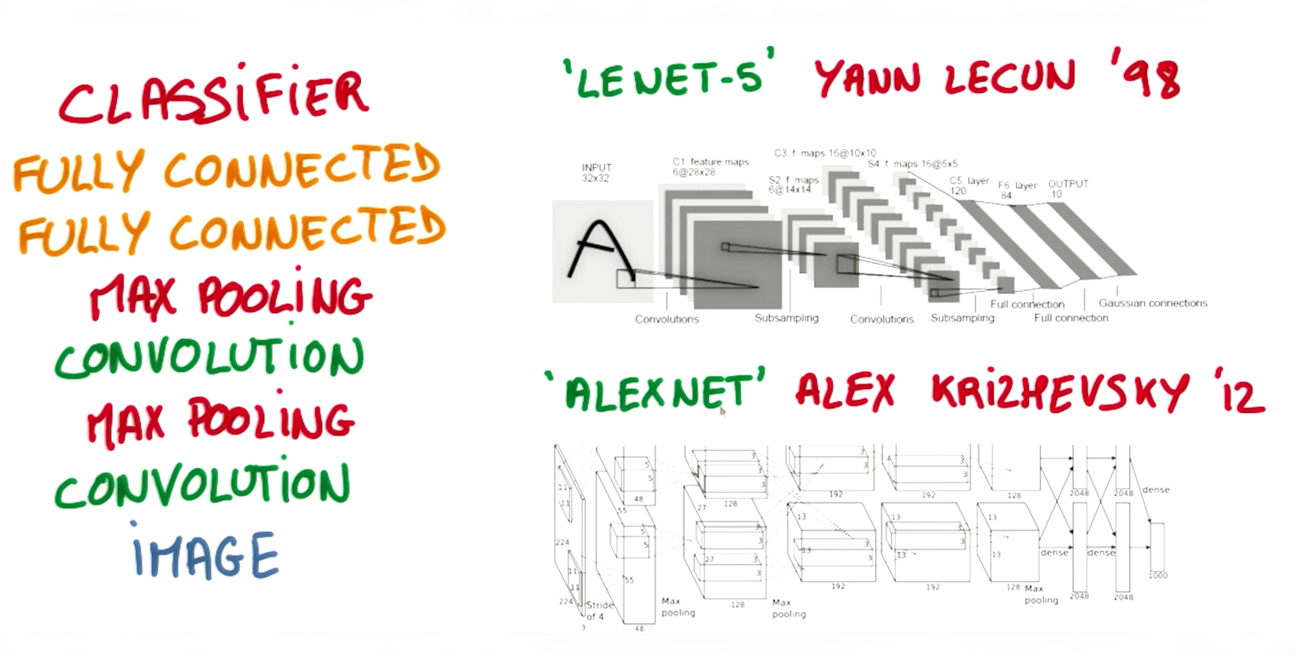
Image from Explore The Design Space video
In the code below, we're creating 3 layers alternating between convolutions and max pooling followed by a fully connected and output layer. The transformation of each layer to new dimensions are shown in the comments. For example, the first layer shapes the images from 28x28x1 to 28x28x32 in the convolution step. Then next step applies max pooling, turning each sample into 14x14x32. All the layers are applied from
conv1
to
output
, producing 10 class predictions.
def conv_net(x, weights, biases, dropout):
    # Layer 1 - 28*28*1 to 14*14*32
    conv1 = conv2d(x, weights['wc1'], biases['bc1'])
    conv1 = maxpool2d(conv1, k=2)

    # Layer 2 - 14*14*32 to 7*7*64
    conv2 = conv2d(conv1, weights['wc2'], biases['bc2'])
    conv2 = maxpool2d(conv2, k=2)

    # Fully connected layer - 7*7*64 to 1024
    fc1 = tf.reshape(conv2, [-1, weights['wd1'].get_shape().as_list()[0]])
    fc1 = tf.add(tf.matmul(fc1, weights['wd1']), biases['bd1'])
    fc1 = tf.nn.relu(fc1)
    fc1 = tf.nn.dropout(fc1, dropout)

    # Output Layer - class prediction - 1024 to 10
    out = tf.add(tf.matmul(fc1, weights['out']), biases['out'])
    return out
Session
Now let's run it!
# tf Graph input
x = tf.placeholder(tf.float32, [None, 28, 28, 1])
y = tf.placeholder(tf.float32, [None, n_classes])
keep_prob = tf.placeholder(tf.float32)

# Model
logits = conv_net(x, weights, biases, keep_prob)

# Define loss and optimizer
cost = tf.reduce_mean(\
    tf.nn.softmax_cross_entropy_with_logits(logits=logits, labels=y))
optimizer = tf.train.GradientDescentOptimizer(learning_rate=learning_rate)\
    .minimize(cost)

# Accuracy
correct_pred = tf.equal(tf.argmax(logits, 1), tf.argmax(y, 1))
accuracy = tf.reduce_mean(tf.cast(correct_pred, tf.float32))

# Initializing the variables
init = tf. global_variables_initializer()

# Launch the graph
with tf.Session() as sess:
    sess.run(init)

    for epoch in range(epochs):
        for batch in range(mnist.train.num_examples//batch_size):
            batch_x, batch_y = mnist.train.next_batch(batch_size)
            sess.run(optimizer, feed_dict={
                x: batch_x,
                y: batch_y,
                keep_prob: dropout})

            # Calculate batch loss and accuracy
            loss = sess.run(cost, feed_dict={
                x: batch_x,
                y: batch_y,
                keep_prob: 1.})
            valid_acc = sess.run(accuracy, feed_dict={
                x: mnist.validation.images[:test_valid_size],
                y: mnist.validation.labels[:test_valid_size],
                keep_prob: 1.})

            print('Epoch {:>2}, Batch {:>3} -'
                  'Loss: {:>10.4f} Validation Accuracy: {:.6f}'.format(
                epoch + 1,
                batch + 1,
                loss,
                valid_acc))

    # Calculate Test Accuracy
    test_acc = sess.run(accuracy, feed_dict={
        x: mnist.test.images[:test_valid_size],
        y: mnist.test.labels[:test_valid_size],
        keep_prob: 1.})
    print('Testing Accuracy: {}'.format(test_acc))
That's it! That is a CNN in TensorFlow. Now that you've seen a CNN in TensorFlow, let's see if you can apply it on your own!